Defining the compliance of electromechanical linear actuators

Modern motion controllers with built-in frequency analyzers allow direct identification of electromechanical actuators … under load … subject to real-word conditions. That in turn may help designers improve stiffness and actuator performance — even to the point of getting higher servo bandwidth.

By Leonid Gannel, Ph.D.  •  Servo engineer  •  Jabil Shemer Motion

Frequency analyzers on motion controllers let engineers identify electromechanical actuators — even subject to real-world conditions. These tools allow analysis of linear actuators as multi-mass models defined by masses of bodies linked by compliant couplings that contribute to system resonances.

Defining the couplings lets designers boost actuator stiffness — in turn boosting actuator performance by increasing its servo bandwidth.

Modeling a motion design with a perfectly stiff plant for the servo design is unrealistic. Motion-design researchers describe the modeling problem it causes as the inertial reduction instability phenomenon. More specifically, this describes how increasing the amplitude of the plant’s Bode with each resonance may lead to low gain (or phase) margin or even loss of stability for velocity (or position) loops.

Now let’s go through an example identification method for defining a three-body actuator — an approach that works for systems modeled with four and more bodies as well. In fact, this method is also valid for actuators with rotating motors. The only difference is that masses and forces must be replaced by rotational inertia (moments of inertia) and moments.

Profiling electromechanical servo actuators — with analysis right at the loaded actuator in a test setup replicating real operating conditions — is the most effective way of quantifying that actuator’s structural features and other characteristics. The mathematical model an engineer gets from this analysis can be used for both velocity and position-loop design and verification of analytical modeling.

Motion controllers with frequency analyzers

Controllers from ACS Motion Control, Elmo, Galil, and others include built-in accurate frequency analyzers that are user friendly. Along with the wide bandwidth of these modern PWM and linear current amplifiers — bandwidths to at least 1 to 2 kHz — the frequency analyzers are indispensable in the study of multi-mass electromechanical actuators.

The presence of resonances due to compliant coupling between motor and load degrades the performance of robot manipulators, CNC machine tools, and X-Y coordinate tables. Vibrations in the low and middle-frequency range limit servo-actuator performance most significantly. Representing the actuator as a set of compliantly coupled bodies helps design engineers identify locations of compliant (low-stiffness) linkages. That in turn may help designers improve the coupling stiffness … and boost actuator performance — even to the point of getting higher servo bandwidth in some cases.

Electromechanical actuator compliance example

The first step of actuator investigation is to analyze plant behavior. Here, the plant is part of the velocity loop from current command to the motor/load/velocity/position. It includes the current amplifier, the motor with linked load, and the position sensor (which in this case is an encoder).

The disturbance (with a harmonic shape, as a rule) is that excited by a current reference signal compared with velocity/position over defined frequency range.  Plant frequency response plotted in a Bode presentation has a logarithmic scale on the horizontal axis with the input signal frequency in Hertz. The ratio of the output position amplitudes (phases) to input motor current in decibels is plotted on the vertical axis.

Consider the specific case of a gantry stage driven by linear electromechanical actuators on its axes. The mathematical description of the actual electromechanical actuator is rather complicated. The actuator has a few resonance phenomena. Each is represented by pairs of anti-resonance (AR) and resonance (R) frequencies with a phase rate up to +180° between them.

For the Bode plots of our example gantry stage, let us choose two resonances for the sake of simplification. Here we must distinguish the three-bodies model for further identification. But because the key resonances are far enough apart, we can apply the superposition principle.

Recall from systems theory that the superposition principle for linear systems states that the net response at a given place and time from two or more inputs is the sum of responses caused by each separate input.

So for our exercise, application of the superposition principle allows simplification of the three-bodies actuator model as a coupled two-body models.

Let’s now use that well-known two-body compliant model to represent the actuator design. For simplification, let’s also ignore internal viscous friction of masses as well as any viscous friction between masses. Refer to the block diagram of linear three-bodies model presented in this piece, as well as the transfer function H₁(s) of first body defined by R₁ and R₂ resonances.

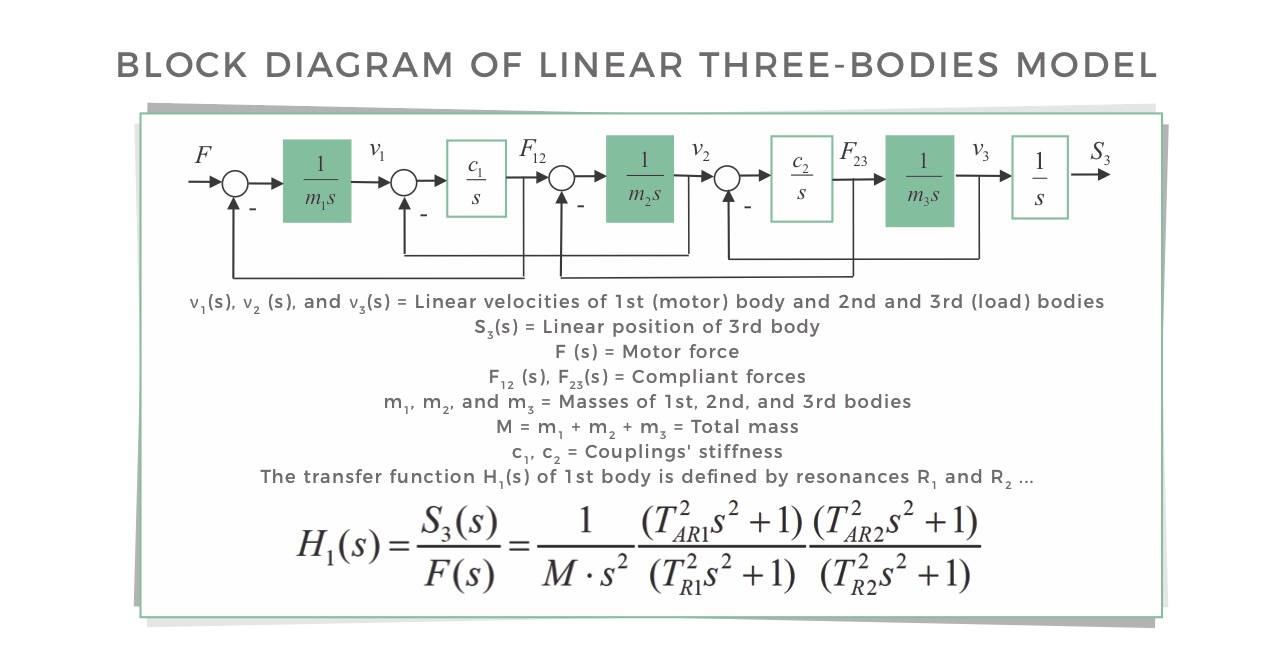
The lower-frequency first resonance R₁ is represented by stiffly coupled first and second bodies with mass m₁₂ = m₁ + m₂ linked with stiffness c₂ to the third body with having m₃ mass. The higher-frequency second resonance R₂ is represented with first and second bodies only linked with c₁ stiffness. The third body is switched off for frequencies higher than resonance R₁ frequency. So that means for transfer functions H₁(s) the T²_AR1 = m₃ · c₂^(-1)  — so the period of AR-frequency of the three-body system is equal to the natural-oscillations period of the third body stiffly coupled to the first and second bodies:

T²_AR2 = m₂ · c₁^(-1)  — the period of AR frequency equal to natural-oscillations period of the second mass with stiff coupling to the first mass and the third mass switched off.

The R-frequency period of the three-bodies model is T²_R1 = (m₁ + m₂ )m₃ c₂^(-1) / (m₁ + m₂ + m₃).

The R-frequency period of the two-mass model is T²_R2 = m₁m₂ c₁^(-1) / (m₁ + m₂) including first and second masses only.

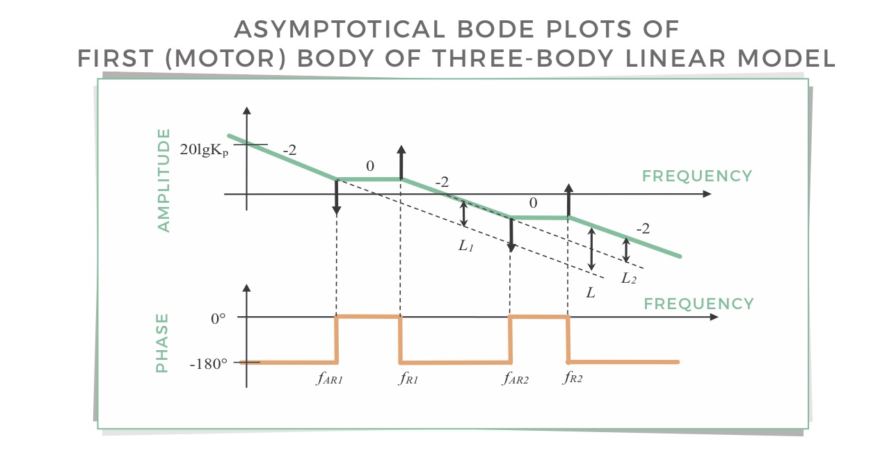
Now consider the Bode plot presented in the figure titled, “Asymptotical Bode plots of first and third-body linear models” of the first body according to transfer functions H₁(s) where a slope of (-2) is equivalent to (-40 dB/decade.

In addition, the slope of the plant-amplitude Bode before the first resonance is defined by total mass M after the first resonance by the sum of first (motor) and second masses — (m₁₂ = m₁ + m₂) and after second resonance by the first mass m₁ only.

That explains the increasing Bode slope by L₁ after the first resonance … and by L₂ after the second resonance.

Let’s use commonly accepted mismatch definitions for second and third bodies so that Y2 = m₂ / m₁ … and Y₃ = m₃ / m₁.

That means that increments of the amplitude Bode L=L₁+L₂ are defined by mismatch ratios as:

L₁ = 20lg[(1 + Y₂ + Y₃) / (1 + Y₂ )] and

L₂ = 20lg(1 + Y₂).

Comparison of the first-body Bode for the structure (refer to the figure titled, “Asymptotical Bode plots of first and third-body linear models”) with the experimental Bode in the screen-capture from the SPiiPLUS FRF Analyzer (from ACS Motion Control for analysis of frequency response functions) confirms that the former is valid to use as a model for further identification.

Calculation of actuator-model parameters

The above equations for periods of anti-resonance with index AR and resonance with index R can be rewritten:

Note that the ratio of frequencies f_R1 to f_AR1 is equal to the square root of the ratio (1 + Y₂ + Y₃) to (1 + Y₂). What’s more, the ratio of f_R2 to f_AR2 is equal to the square root of (1+Y₂). Both AR and R frequencies maybe determined more accurately from the experimental phase Bode but not from the amplitude Bode — especially in situations with low mismatches.

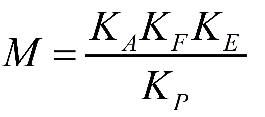
Except for AR and R frequencies, the total actuator mass M can also be calculated from the experimental Bode. Here, the total Plant Gain 20log K_P is found from the amplitude Bode at the angular frequency of 1 rad/sec. In fact, we can find three things from motor data sheets and the ACS Motion Control controller we use to explore our example gantry setup:

1) Gains of plant components as current amplifier K_A in A_pk/bit

2) The motor force constant K_F in N/A_pk

3) Position resolution K_E in counts/m

So total mass M in kg is:

Case in point: Specifics on our gantry-table example

As an example, consider the axis on our XY gantry table. Assume it sports a linear ironcore motor and linear position encoder controlled from motion controller — the ACS SPiiPlusCM with an internal three-phase sinusoidal PWM power amplifier. As can be seen from the experimental plant Bode (shown in the Bode-plat figure) the actuator has two highly pronounced resonances. That means that the three-bodies model work for further identification. Note that we ran our experiments with nonzero velocity to avoid registering the effects of friction at low-frequency ranges. Let’s determine the parameters of the model according to the proposed method.

Refer to the figure titled, “Gantry case-study calculations” for initial data as well as the data derived from the experimental Bode. These calculations indicate that the compliant coupling leading to the first lower-frequency resonance is between the body with mass m₁ + m₂ = 452 kg and the third body with mass m₃ = 158 kg. In addition, compliant coupling leading to second higher-frequency resonance is between the first body with mass body m₁ = 161 kg and the second with m₂ = 291 kg.

What does this all mean? Essentially it indicates that the source of the first resonance is radial compliance in the Y linear bearing. The source of the second resonance is axial compliance in the X linear bearing. In some such cases, design engineers can work with linear-systems manufacturers to address such compliant behavior — for example, by increasing preload on the linear assembly.

Jabil Shemer Motion | www.shemer.com • ACS Motion Control | acsmotioncontrol.com