
One of the first steps in sizing any type of linear guide or drive component is to determine the required motion profile. The motion profile is simply a way to define and graphically depict how the component should achieve the specified travel, in terms of velocity and time.
The motion profile is the basis for determining the required acceleration (and deceleration) of the system. The acceleration and deceleration portions of the motion profile impart forces on the system (F = ma) that must be accounted for when sizing and selecting the guide or drive components. The required acceleration also plays an important role in determining the torque required from the motor and is a key component of motor sizing.
The vast majority of linear motion applications require either a triangular or a trapezoidal motion profile, or a combination of the two. A triangular motion profile is most often used for traveling from one point to another in the shortest amount of time. The constant velocity phase of a triangular move profile is very short and is often disregarded, with the assumption that the system accelerates to a maximum velocity and then immediately decelerates to zero. General pick-and-place and transport applications often use triangular motion profiles.
A trapezoidal motion profile is used when a specific maximum velocity should be sustained for some amount of time. Dispensing, machining, and printing applications typically use trapezoidal motion profiles because they include a time where the velocity is steady, with no acceleration or deceleration.
 Think of the difference between triangular and trapezoidal motion profiles as the difference between sprinting and cross-country running. The goal of a sprinter is to reach the finish line as quickly as possible, much like a linear motion system with a triangular motion profile. Cross country runners, on the other hand, run at a constant pace (velocity) for the majority of the time, much like a linear motion system operating with a trapezoidal motion profile.
How to create a triangular motion profile
If the application calls for minimizing the time it takes to reach the target position, it will typically use a triangular motion profile, and the application parameters will specify the total distance to be traveled and the time allowed for the move. In this example, we’ll assume the application requires a travel of 1.25 m in 0.75 s.
With total distance (1.25 m) and total time (0.75 s) specified, the first step in creating the triangular motion profile is to determine the average velocity, which is simply total distance divided by total time.
vavg = dt/tt
vavg = 1.25 m/0.75 s
vavg = 1.67 m/s
In order to create the motion profile, we also need to know the maximum velocity, which will be the height of the triangle. A common assumption for triangular motion profiles is that the times for acceleration and deceleration are equal, which means the maximum velocity is simply twice the average velocity.
vmax = 2*vavg
vmax = 2*1.67 m/s
vmax = 3.34 m/s
Now, we can plot the triangular motion profile.

The X axis represents travel time, which is a total of 0.75 s. The Y axis represents velocity, which ranges from 0 m/s at the beginning of the move, to the maximum velocity of 3.34 m/s. Since this is a triangular motion profile with equal acceleration and deceleration phases, the maximum velocity (3.34 m/s) occurs exactly halfway between 0 s and 0.75 s, at 0.38 s.
How to create a trapezoidal motion profile
When a trapezoidal motion profile is required, the application parameters will typically include the maximum velocity and either the distance or the time that maximum velocity should be sustained. But recall that motion profiles are defined in terms of velocity and time, so if you’re working from application parameters that specify velocity and distance, you’ll need to determine the required time for each phase of the move. Here’s an example…
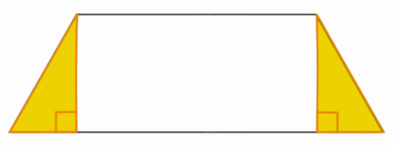
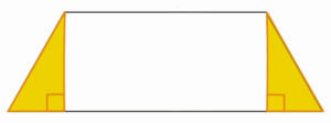
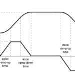
We’ll break the motion profile into three phases: acceleration, constant velocity, and deceleration, which are represented on the trapezoid as a triangle, a rectangle, and a triangle.
The simplest case of a trapezoidal motion profile is commonly referred to as a “ 1/3, 1/3, 1/3” profile, because each phase — acceleration, constant velocity, and deceleration — takes 1/3 of the total time. In a past blog post — How to calculate velocity — we explained how to work with 1/3, 1/3, 1/3 trapezoidal motion profiles, so in this example, we’ll assume that the times for acceleration and deceleration are equal, but shorter than the time for constant velocity.
First, let’s define the constant velocity portion of the move, which is the rectangular portion of the trapezoid. Recall that velocity equals distance divided by time. Rearranging for time, we can use this basic equation to determine the time for the constant velocity portion of the move. In this application, we’ll assume the maximum (constant) velocity is 0.5 m/s and the constant velocity will be sustained for 2 m, so the time for constant velocity is 4 s.
tc = dc/vmax
tc = 2 m/0.5 m/s
tc = 4 s
Next, let’s define the acceleration and deceleration portions of the motion profile, which, in the trapezoidal figure, are the right triangles on each side of the rectangle. Let’s assume that the application parameters specify that the distance for acceleration is 0.1 m and for deceleration is 0.1 m. But to plot the motion profile, we need to determine how much time is used for acceleration and deceleration.
In the previous post, we derived the formula for total distance traveled in a trapezoidal motion profile, based on the areas of the two triangular portions (½*b*h) and the area of the rectangular portion (b*h).
dt = (½*b*h)+ (b*h) + (½*b*h)
Where b is the base (time) and h is the height (velocity).
dt = (½*ta*vmax) + (tc*vmax) + (½*td* vmax)
The application parameters tell us that the maximum velocity is 0.5 m/s, and we determined that the time for constant velocity is 4 s. We also know the total distance for the move is 0.1 m for acceleration, 2 m for constant velocity, and 0.1 m for deceleration, so the total distance, dt, is 2.2 m.
Plugging these values into the equation for total distance, we get:
2.2 m = (½*ta*0.5 m/s) + 4 s*0.5 m/s + (½*td*0.5 m/s)
2.2 m = ta*0.25 m/s + 2 m + td*0.25 m/s
0.2 m = ta*0.25 m/s + td*0.25 m/s
0.2 m = 0.25 m/s * (ta+td)
0.8 s = ta+td
We established earlier that the times for acceleration and deceleration (ta and td) were equal, so in this case, ta = td = 0.4 s.
ta = td = 0.4 s
Now we can plot the trapezoidal motion profile.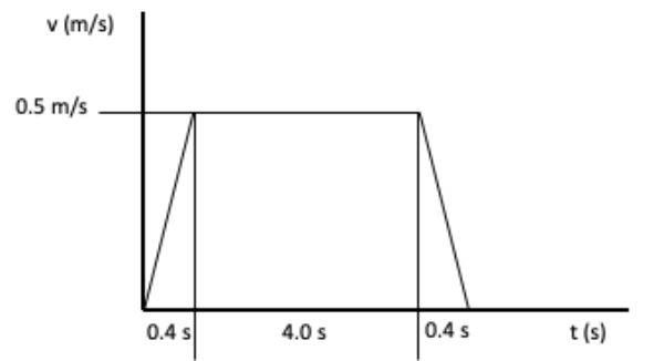
Although there do exist more complex motion profiles than the triangular and trapezoidal versions described here, these two basic forms provide good approximations for most linear motion systems. And if you understand the relationships between time, distance, and velocity, along with basic trigonometric equations for triangles, you can derive even complex motion profiles. Then the motion profile can be used to determine the required acceleration and deceleration rates for the application and whether the defined move parameters meet the application’s requirements.
Feature image credit: Varedan Technologies

Leave a Reply
You must be logged in to post a comment.